lecture11

Lecture 11

Dynamic Instability of the Microtubule

What is the timescale of fluctuations? ()

A good guess would be that it depends only on the two rates which we are aware of - the attach and detach rates.

Dynamic Instability in microtubule-like filaments

  • Microtubules have dynamic instability
    • One end of the microtubule is composed of stable (GTP) monomers while the rest of the tubule is made up of unstable (GDP) monomers.
      • The GTP end comprises a cap of stable monomers.
    • Random fluctuations either increase or decrease the size of the cap.
      • This results in 2 different dynamic states for the microtubule.
        • Growing: cap is present
        • Shrinking: cap is gone

Lets define some parameters to describe how the microtubule switches between these to states and also how it behaves once in a state.

If we are in the growth state then monomers may be added to the filament.

If we are in the shrinkage state then monomers may be released from the filament.

The microtubule switches between these two states.

If we were to plot the length of the microtubule as a function of time it would look something like the following:

Lets now try to write a model that can describe how this occurs.

Dynamic Model

Lets define as being the fraction of time spent in the growth state. Hence the fraction of time spent in shrinkage state is then .

Similar to what we have done in previous lectures, our dynamic model is expressed as the following:

The fractions and can expressed in terms of the rates we defined above.

  • Growth is bounded if .
  • Growth is unbounded if .

Stochastic Model

Now lets think in terms of probabilities. We need to assign probabilities to being in either a growth or shrinkage state with a certain number of links .


The probability of being a microtubule with links is .
If , .
If , .

Growth Rate

For

For

In a bounded state we can solve for the stationary distribution of by setting the time derivatives equal to zero.

For

For

If we repeat this process for we notice a pattern emerge.

We can solve for by normalizing the probability distribution.

This is not quite a (exponential) geometric distribution. A geometric distribution looks like the following:

Whereas in our case we have the following relationships:

Notice that when we solved for the series we assumed in order for the series to converge, and so this is in fact a bounded state.

Written with StackEdit.

cellstretch_notes

Simulation Notes: Stretchable Cells

Simulation Set-up

  • Reflective boundary on the left.
  • Absorbing boundary on the right.
  • Cells are always connected, cells may stretch and contract.
    • The number of cells is varied.
    • The amount by which a cell can stretch is varied.
      • cellstretch refers to the maximum number of additional lattice points a cell may occupy.
  • Cells are initialized along the reflective boundary and all only occupy one lattice point.

Mean First Passage Time

Hypothesis

  • The mean passage time will increase exponentially as the number of cells in the simulation increases.
  • The strength of the exponential will decrease if the cells are allowed to stretch more.

Results

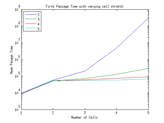
wiggle_1
The box indicates the value of cellstretch for that set of data.

  • In the one cell case we recover the same result as the single cell diffusion simulations. The mean passage time is time steps.
  • For to our hypothesis seems to be on the right track.
    • I am unsure as to the cause of the kink in the exponential increase which occurs at for all cases.
      • I believe it has something to do with the fundamental difference between 1 and multiple cell diffusion. When then the cells must stay connected and diffuse together whereas in the 1 cell case there is no such constraint.
  • Our hypothesis that increasing cellstretch will decrease the strength of the exponential increase is incorrect.
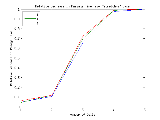
    • I am surprised by how the benefit of being able to stretch more quickly decreases.

Below is the relative decrease in mean passage time with respect to the cellstretch = 2 case.
wiggle_2

Written with StackEdit.

1d_diffusion_notes

1D Diffusion Notes

1 Cell Diffusion with No State Switching

Prediction

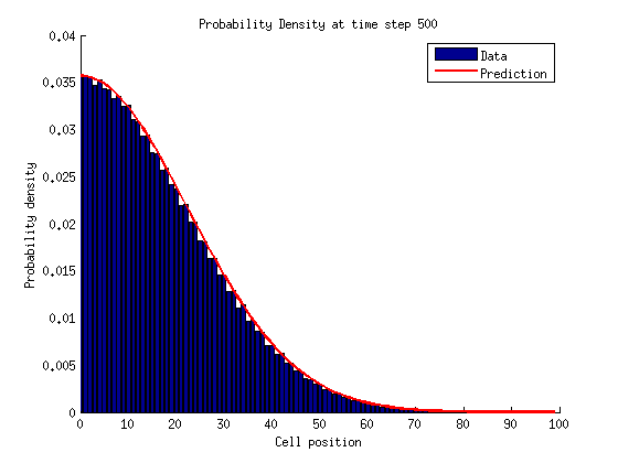
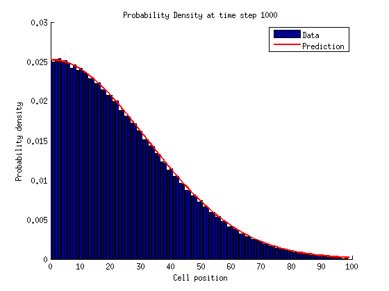
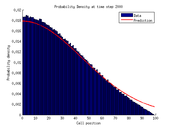
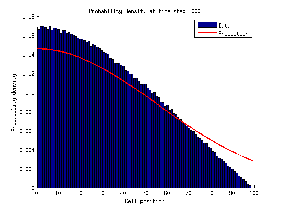
The probability density for cell location given a time should look like a normal distribution. As time increases this prediction becomes less accurate since more and more particles get absorbed at the right side boundary.

The extra factor of two in is because of the reflective boundary at the origin. In an 1D random walk so , therefore , and .

Results

At small times the data is very much inline with prediction.

pdf_0500
pdf_1000

At large times the data starts to diverge from a normal distribution as more and more cells are absorbed.

pdf_2000
pdf_3000

Prediction

is the probability density of the first passage time. It is expressed as the following:

This equation has a solution for our set of initial and boundary conditions. In the large time limit this solution can be expressed as:

In the following plots only the first term, , from the series is used.

Update
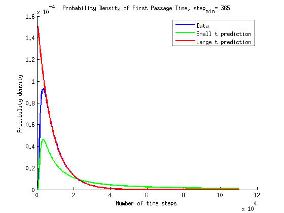
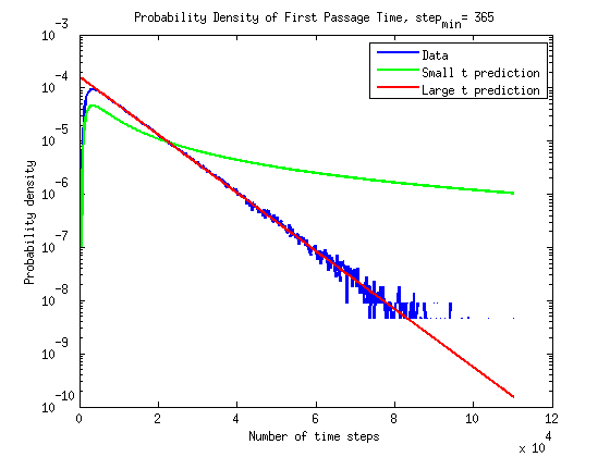
I have added a short time prediction for to the plots below. We observed that at short times looks like a normal distribution. Hence an appropriate approximation for the small time behavior of can be calculated from the normal distribution.

Therefore the short time approximation is the following:

Results - Update

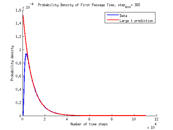
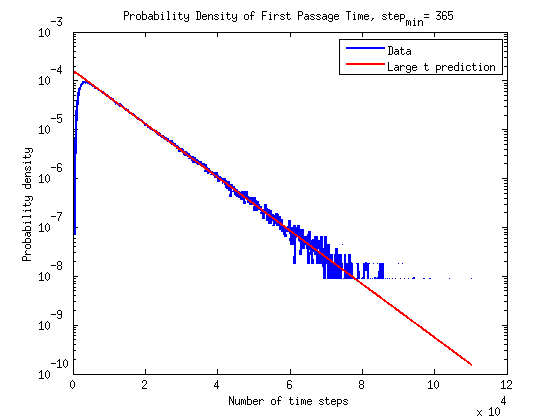
The results are plotted here on a normal scale and on a semilog scale. The prediction at large times does seems to be in agreement with the simulations.

Update 2, I have added the small time prediction to the plots. At small times it does seems to be in agreement with the simulations. The semilog plot illustrates that the the exponential increase in is well described by the small time approximation.

time_pdf_3_histfix

time_pdf_semilog3_histfix

Update 1, I have since gone back and remade the plots as a histogram. In creating the histograms I weight the probability density in each bin by the width of the bin to ensure that the whole probability density is properly normalized.

time_pdf_2_histfix

time_pdf_semilog2_histfix

Old Plots
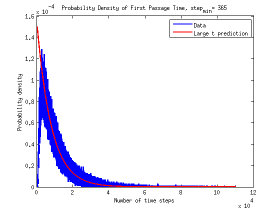
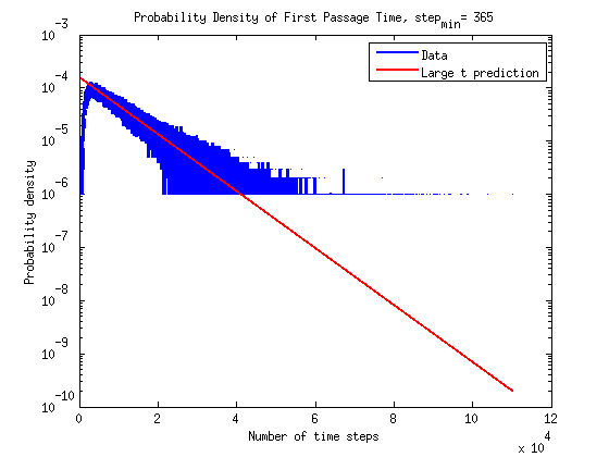
I believe the thickness of the band in the data is due in part because of the large time scale plotted and that on small timescales there is lots of variation in the probability density.

time_pdf_1
time_pdf_semilog1

Written with StackEdit.