Lecture 8
Bacteria Forward Motion
How do bacteria achieve forward motion?
Bacteria have flagella that drive their propulsion. Bacteria flagella move in a corkscrew pattern. Flagella do not flap back and forth like a paddle. Why do flagella corkscrew instead of flapping in order to achieve forward motion? The last two minutes of this video illustrates why a bacteria would want to have its flagella move in a corkscrew instead of in a rowing motion.
This has to do with the Reynolds Number associated with the bacteria’s environment. Reynolds number may be expressed as
is the density of the fluid, is the viscosity of the fluid, is the length scale of the object in the fluid, and is its velocity.
Reynolds Number Discussion
We can gain some insight into the dynamics of a bacteria’s motion by calculating its Reynolds number and comparing it to other cases.
In Water
and
Fish
-
Bacteria
-
In Molasses
- Fish
From the bacteria’s perspective moving through water is analogous to a macroscopic object moving through syrup. Hence, observing macroscopic objects in very viscous fluids (like molasses) can give us insight into bacteria motion since they also experience an environment with very low Reynolds number.
Reynolds Number Experiment
Rods in Viscous Fluids
Observing how rods fall in a viscous fluid can give us insight into how bacteria move. The video above also gives examples of rods falling through viscous fluids (skip the first minute to get to the relevant parts). The video shows examples of rods falling horizontally, vertically and diagonally.
The drag force on an object is ; is the drag coefficient and depends on the length scale of the object and the fluid that it is in.
A rod falling vertically feels half of the drag froce that an identical rod falling horizontally experiences. This is because of the difference in the drag coefficients between the two scenarios.
A rod falling diagonally will feel a drag force which has a component due to horizontal drag as well as vertical drag. The drag force in the perpendicular direction will be greater in magnitude than that in the parallel direction, . This will result in a net motion of the rod moving both down and to the side because of the inequality in the two drag components.
Comparison to Bacteria
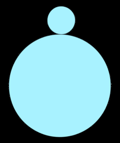
We want to examine how the flagellum of a bacteria compares to the falling rod.

For our purposes lets only focus on the flagellum, not on the accompanying cilia diagram.
Assume that the flagellum is rotated a a frequency . Lets consider a small section of the flagellum with length . The whole flagellum moves in a corkscrew with angular velocity the motion traces out a circle of diameter and the flagellum makes an angle with the passive part. The angle is then the angle the small section makes normal to the basal body.
The forces acting on the small section is analogous to the forces acting on the diagonally falling rod except that gravity is negligible in this case. The velocity of the small section is radially outwards. It also experiences two drag forces, one point parallel to the section and one point perpendicular .
and are the components of the velocity vector pointing in the respective directions.
Likewise, the drag coefficients are the same as those of the rod falling vertically or horizontally.
The propulsive force that this small section exerts is equal to the components of the two drag forces that point in the direction of forward motion (normal to the basal body).
The total propulsive force of the whole flagellum is the sum of all the contributions from each small section.
Lets estimate the terminal velocity of a bacteria.
Approximate the bacteria as a rod of length moving at speed . At terminal velocity, .
For a typical bacteria this equates to a terminal velocity which is very close to observed velocities .
Flagellar Efficiency
Purcell wrote a paper deriving the efficiency of flagellar propulsion.

In this case we assume that cell body is spherical and rotates with angular velocity and the flagellum rotates at angular velocity . The relative anglular velocity between the body and flagellum is .
Next we want to calculate to forces and torques acting on both the body and the flagellum.
Forces and Torques
Cell Body
and are drag coefficients. and .
Flagellum
Rotation of the flagellum causes a drag force and forward motion also causes a drag torque. In Purcell’s paper it was shown that . So our system of equations simplifies to the following:
The constants scale as… , , .
Balance Forces and Torques
If the bacteria’s angular and linear velocities constant then the net force and torque on the whole bacteria must be zero. This leads to the following two equations:
We can equate with the propulsive that we calculated earlier and likewise we can think of as the analogous propulsive torque.
In summary we have three equations
If we assume that and then the above equation simplifies to
Written with StackEdit.