Lecture 11

Dynamic Instability of the Microtubule

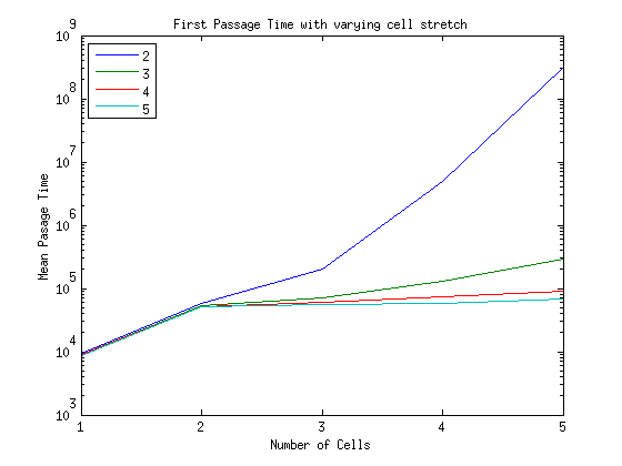
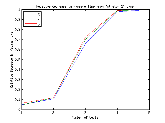
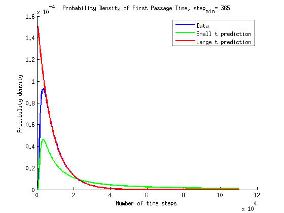
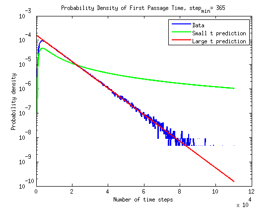
What is the timescale of fluctuations? ($\tau$)

A good guess would be that it depends only on the two rates which we are aware of - the attach and detach rates.

$$\tau \approx \frac{1}{\alpha}+\frac{1}{\mu} \approx \frac{2}{\mu}$$

Dynamic Instability in microtubule-like filaments

• Microtubules have dynamic instability
  
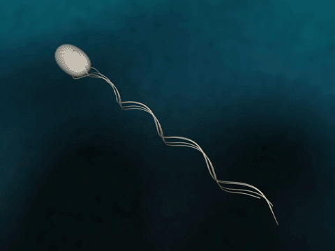
  • One end of the microtubule is composed of stable (GTP) monomers while the rest of the tubule is made up of unstable (GDP) monomers.
    
    • The GTP end comprises a cap of stable monomers.
  • Random fluctuations either increase or decrease the size of the cap.
    
    • This results in 2 different dynamic states for the microtubule.
      
      • Growing: cap is present
      • Shrinking: cap is gone

Lets define some parameters to describe how the microtubule switches between these to states and also how it behaves once in a state.

$$g \equiv \text{switch from shrinking to growing rate} \\ s \equiv \text{switch from growing to shrinking rate} \\ $$

If we are in the growth state then monomers may be added to the filament.

$$\alpha \equiv \text{attach rate}$$

If we are in the shrinkage state then monomers may be released from the filament.

$$\mu \equiv \text{detach rate}$$

The microtubule switches between these two states.

If we were to plot the length of the microtubule as a function of time it would look something like the following:

Lets now try to write a model that can describe how this occurs.

Dynamic Model

Lets define $f$ as being the fraction of time spent in the growth state. Hence the fraction of time spent in shrinkage state is then $1-f$.

Similar to what we have done in previous lectures, our dynamic model is expressed as the following:

$$\bar{n}(t)=\alpha(ft)-\mu[(1-f)t]+n_0$$

The fractions $f$ and $1-f$ can expressed in terms of the rates we defined above.

$$f = \frac{g}{g+s} \\ 1-f=\frac{s}{g+s} \\ \Rightarrow \bar{n}(t)=\left[\frac{\alpha g}{g+s}-\frac{\mu s}{g+s}\right]t + n_0$$

• Growth is bounded if $\alpha g<\mu s$.
• Growth is unbounded if $\alpha g>\mu s$.

Stochastic Model

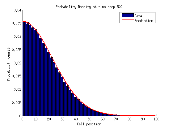
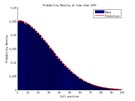
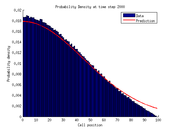
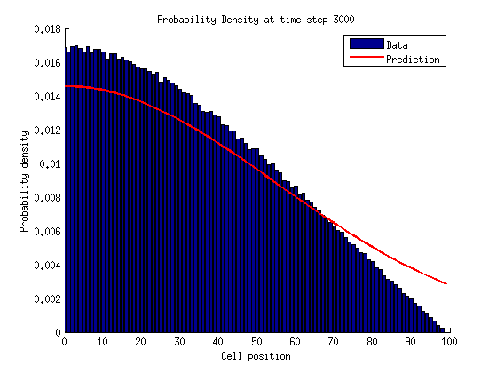
Now lets think in terms of probabilities. We need to assign probabilities to being in either a growth or shrinkage state with a certain number of links $n$.

$p(n,+)\equiv q_n = \text{probability of being in growth state}$
$p(n,-)\equiv r_n = \text{probability of being in shrinkage state}$

The probability of being a microtubule with $n$ links is $p_n$.
If $n=0$, $p_n = q_0$.
If $n\geq1$, $p_n=q_n+r_n$.

Growth Rate

$$\frac{dp(n,+)}{dt}=\frac{dq_n}{dt}$$

For $n\geq 1$

$$\frac{dq_n}{dt} = \alpha \ q_{n-1}-\alpha \ q_n - s \ q_n + g \ r_n \\ \frac{dr_n}{dt} = \mu \ r_{n+1}-\mu \ r_n+s \ q_n -g \ r_n$$

For $n=0$

$$\frac{dq_0}{dt}=\mu \ r_1-\alpha \ q_0$$

In a bounded state we can solve for the stationary distribution of $p_n$ by setting the time derivatives equal to zero.

For $n=0$

$$\Rightarrow r_1=\frac{\alpha}{\mu}q_0=\lambda q_0 \\ \lambda \equiv \frac{\alpha}{\mu}$$

For $n=1$

$$0 = \alpha \ q_0-\alpha \ q_1 - s \ q_1 + g \ r_1 \\ 0 = \mu \ r_2-\mu \ r_1+s \ q_1 -g \ r_1 \\ x \equiv \lambda \frac{\mu+g}{\alpha+s} \\ \Rightarrow q_1=x \ q_0, \ \ r_2 = \lambda \ x \ q_0$$

If we repeat this process for $n=2,3,4,...$ we notice a pattern emerge.

$$q_n = x^nq_0 \\ r_n=x^{n-1} \lambda \ q_0$$

We can solve for $q_0$ by normalizing the probability distribution.

$$1=\sum_{n=0}^\infty p_n = q_0 + \sum_{n=1}^\infty (q_n+r_n) \\ 1=q_0\left[\frac{1-x+x+\lambda}{1-x}\right] \\ q_0 = \frac{1-x}{1+\lambda}$$

$$p_n = \begin{cases} q_0, & n = 0 \\ q_0 x^n \left(1+\frac{\lambda}{x}\right), & n\geq1 \end{cases}$$

This is not quite a (exponential) geometric distribution. A geometric distribution looks like the following:

$$p_n=(1-\lambda)\lambda^n \\ \frac{p_{n+1}}{p_n}=\lambda$$

Whereas in our case we have the following relationships:

$$\frac{p_1}{p_0}=x+\lambda, \ \ \ \frac{p_{n+1}}{p_n}=x \ \ \text{for} \ n\geq1$$

Notice that when we solved for the series we assumed $x<1$ in order for the series to converge, and so this is in fact a bounded state.

Written with StackEdit.

cellstretch_notes

Simulation Notes: Stretchable Cells

Simulation Set-up

• Reflective boundary on the left.
• Absorbing boundary on the right.
• Cells are always connected, cells may stretch and contract.
  
  • The number of cells is varied.
  • The amount by which a cell can stretch is varied.
    
    • cellstretch refers to the maximum number of additional lattice points a cell may occupy.
• Cells are initialized along the reflective boundary and all only occupy one lattice point.

Mean First Passage Time

Hypothesis

• The mean passage time will increase exponentially as the number of cells in the simulation increases.
• The strength of the exponential will decrease if the cells are allowed to stretch more.

Results

The box indicates the value of cellstretch for that set of data.

• In the one cell case we recover the same result as the single cell diffusion simulations. The mean passage time is $10^4$ time steps.
• For $N=2$ to $N=5$ our hypothesis seems to be on the right track.
  
  • I am unsure as to the cause of the kink in the exponential increase which occurs at $N=2$ for all cases.
    
    • I believe it has something to do with the fundamental difference between 1 and multiple cell diffusion. When $N\geq2$ then the cells must stay connected and diffuse together whereas in the 1 cell case there is no such constraint.
• Our hypothesis that increasing cellstretch will decrease the strength of the exponential increase is incorrect.
  
  • I am surprised by how the benefit of being able to stretch more quickly decreases.

Below is the relative decrease in mean passage time with respect to the cellstretch = 2 case.

Written with StackEdit.

1D Diffusion Notes

1 Cell Diffusion with No State Switching

$P(x|t)$

Prediction

The probability density for cell location given a time $t$ should look like a normal distribution. As time increases this prediction becomes less accurate since more and more particles get absorbed at the right side boundary.
$$P(x|t) = \frac{2}{\sqrt{2\pi\sigma^2}} e^{-x^2/2\sigma^2} \\ \sigma^2 = 2Dt$$
The extra factor of two in $P(x|t)$ is because of the reflective boundary at the origin. In an 1D random walk so $\left<x\right> = 0$, therefore $\sigma^2 = \left<x^2\right>$, and $\left<x^2\right> = Nb^2$.
$$\Rightarrow 2Dt = Nb^2 \\ t = N \Delta t \\ \Rightarrow D = \frac{b^2}{2\Delta t}$$

Results

At small times the data is very much inline with prediction.

At large times the data starts to diverge from a normal distribution as more and more cells are absorbed.

$P(t)$

Prediction

$P(t)$ is the probability density of the first passage time. It is expressed as the following:
$$P(t) = -D \frac{\partial P(x|t)}{\partial x} |_{x=L}$$
This equation has a solution for our set of initial and boundary conditions. In the large time limit this solution can be expressed as:
$$P(t) = \frac{2D}{L^2} \sum_{m=1}^{\infty} \beta_m e^{-\beta_m^2 D t / L^2} \sin\left(\beta_m \frac{x}{L}\right) |_{x=L}$$
In the following plots only the first term, $m=1$, from the series is used.

Update
I have added a short time prediction for $P(t)$ to the plots below. We observed that at short times $P(x|t)$ looks like a normal distribution. Hence an appropriate approximation for the small time behavior of $P(t)$ can be calculated from the normal distribution.
$$P(x|t) = \frac{2}{\sqrt{2\pi\sigma^2}} e^{-x^2/2\sigma^2} \Rightarrow \frac{\partial P(x|t)}{\partial x} = \frac{-2x}{\sigma^2\sqrt{2\pi\sigma^2}}e^{-x^2/2\sigma^2} \\ $$
Therefore the short time approximation is the following:
$$P(t) = \frac{x}{t\sqrt{2\pi\sigma^2}}e^{-x^2/2\sigma^2} |_{x=L}$$

Results - Update

The results are plotted here on a normal scale and on a semilog scale. The prediction at large times does seems to be in agreement with the simulations.

Update 2, I have added the small time prediction to the plots. At small times it does seems to be in agreement with the simulations. The semilog plot illustrates that the the exponential increase in $P(t)$ is well described by the small time approximation.

Update 1, I have since gone back and remade the plots as a histogram. In creating the histograms I weight the probability density in each bin by the width of the bin to ensure that the whole probability density is properly normalized.

Old Plots
I believe the thickness of the band in the data is due in part because of the large time scale plotted and that on small timescales there is lots of variation in the probability density.

Written with StackEdit.

Lecture 10

Dynamics: Filament Polymerization

Polymerization at Both Ends (cont.)

Actin

Unlike microtubules, actin does not have the same critical concentration for the “$+$” and “$-$” ends.
$$c^*_+ \neq c^*_-$$
Plotting $\frac{dn_\pm}{dt}$ as a function of $c$ will illustrate a different phase space than that of microtubules.
Assume that $c^*_+ < c^*_-$, this gives us the following relationships between $c$ and $\frac{dn_\pm}{dt}$.
$$\ \ \ \ \ \ \ \ \ \ c < c^*_+ \ \Rightarrow \ \frac{dn_+}{dt}<0 \text{ and } \frac{dn_-}{dt} < 0 \ \ [1]\\ c^*_+< c < c^*_- \ \Rightarrow \ \frac{dn_+}{dt}>0 \text{ and } \frac{dn_-}{dt} < 0 \ \ [2]\\ \ \ \ \ \ \ \ \ \ \ c < c^*_+ \ \Rightarrow \ \frac{dn_+}{dt} > 0 \text{ and } \frac{dn_-}{dt} > 0 \ \ [3]$$
The three relationships above yield 3 different phases for actin.

$[1]$: Both ends shrink
$[2]$: The $+$ end grows, $-$ end shrinks
$[3]$: Both ends grow

For some value of $c$ within the regime of $[2]$ the rate at which the $+$ end grows equals the rate the $-$ end shrinks. This concentration is called the treadmilling concentration $c_T$.
$$c=c_T \Rightarrow \frac{dn_+}{dt} = \frac{dn_-}{dt}$$

Simple treadmilling animation

For actin, $c_T\approx 0.16\mu M$. Both ends grows and shrink at the same rate resulting in the length of the actin remaining fixed. The system is in a steady state, however it is not in thermodynamic equilibrium because the filaments are constantly shifting. We can derive $c_T$ by noting that the total number of filaments $n$ remains constant.
$$\frac{dn}{dt} = 0 \\ \frac{dn}{dt} = \frac{d(n_++n_-)}{dt} = \frac{dn_+}{dt} + \frac{dn_-}{dt} \\ \Rightarrow \frac{dn_+}{dt} = - \frac{dn_-}{dt} \neq 0 \\ k_+ c_T - \mu_+ = -k_- c_T + \mu_- \\ \Rightarrow c_T = \frac{\mu_+ + \mu_-}{k_+ + k_-}$$

Problems with the Model

Our model, given by the rate equation has a couple of problems.
$$\text{Rate Equation: } \frac{dn}{dt} = \alpha-\mu$$

• Nothing in this model says that $n$ cannot be negative.
  
  • Physically, the number of filaments must be zero or positive.
• At small values of $n$ a continuous differential equation is no longer realistic. We can no longer approximate changes in $n$ as being continuous.

In order to try to solve these problems in our model we take a probabilistic approach. Let’s examine what may happen to a filament during small interval of time $\Delta t$ and their respective probabilities.

1. Add a filament: $\ \ \ \ \ \ \ \ p(n \rightarrow n+1) = \alpha\Delta t$
2. Subtract a filament: $\ p(n \rightarrow n-1) = \mu\Delta t$
3. Nothing happens: $\ \ \ \ p(n\rightarrow n) \ \ \ \ \ \ \ = 1 - (\alpha-\mu)\Delta t$

Using these relations we can formulate the probability that at some time $t+\Delta t$ the actin has $n$ filaments, $p_n(t+\Delta t)$. There are three different ways to get to a state with $n$ filaments: add 1 filament, subtract 1 filament, and the actin had $n$ filaments and nothing changed. Quantitatively this can be expressed as the following:
$$p_n(t+\Delta t) = p_{n-1}(t)\alpha\Delta t+ p_{n-1}(t)\mu\Delta t + p_n(t)(1 -\alpha\Delta t-\mu\Delta t)$$
This can apply to all values of $n$ except for edge cases. For example, at $n=0$ the probability of having zero filaments is
$$p_0(t+\Delta t) = p_1(t)\mu\Delta t + p_0(t)(1-\alpha\Delta t).$$

We can re-write the two equations above to show how the probabilities vary as a function of time.
$$\frac{p_n(t+\Delta t) - p_n(t)}{\Delta t} = \dot{p}_n\\ $$
$\text{for }\ n>0: \ \ \dot{p}_n=\alpha \ p_{n-1}+ \mu \ p_{n+1} - (\alpha+\mu)p_n$
$\text{for }\ n=0: \ \ \dot{p}_0=\mu \ p_1-\alpha \ p_0$

The two above equations dictating the behavior of $\dot{p}_n$ are called the (stochastic) Master Equation.

Expectation Value

We can calculate the expectation value (mean) of $n$ using the following formula:
$$\left<n\right> \equiv \bar{n} = \sum_{n=0}^\infty n \ p_n \\ \frac{d\bar{n}}{dt}=\frac{d}{dt} \sum_{n=0}^\infty n \ p_n = 0 \cdot\frac{dp_0}{dt}+\sum_{n=1}^\infty n \ \frac{p_n}{dt} \\ \frac{d\bar{n}}{dt}=\alpha\sum_{n=1}^\infty n\ p_{n-1} + \mu\sum_{n=1}^\infty n\ p_{n+1} -(\alpha+\mu)\sum_{n=1}^\infty n \ p_n$$
The expression for $\frac{d\bar{n}}{dt}$ can be simplified by rewriting the different summation terms. By changing the summation index and by noting that for $n=0 \rightarrow n \ p_n=0$ we can make a few simplifications.

For the first summation term:
$$\sum_{n=1}^\infty n\ p_{n-1} \rightarrow \sum_{n'=0}^\infty(n'+1)p_{n'} = \sum_{n'=0}^\infty n' \ p_{n'} + \sum_{n'=0}^\infty p_{n'} \\ = \bar{n} + 1$$

For the second summation term:
$$\sum_{n=1}^\infty n\ p_{n+1} \rightarrow \sum_{n=0}^\infty n\ p_{n+1} \rightarrow \sum_{n'=1}^\infty (n'-1)p_{n'} \\ = \sum_{n'=1}^\infty n'\ p_{n'} - \sum_{n'=1}^\infty p_{n'} \\ = \bar{n} - (1-p_0)$$

For the third dummation term:
$$\sum_{n=1}^\infty n \ p_n \rightarrow \sum_{n=0}^\infty n \ p_n \\ = \bar{n}$$

This simplifies $\frac{d\bar{n}}{dt}$ to the following:
$$\frac{d\bar{n}}{dt} = \alpha\ \bar{n}+\alpha+\mu\ \bar{n}-\mu+\mu \ p_0 -\alpha \ \bar{n}- \mu \ \bar{n} \\ \Rightarrow \alpha-\mu+\mu \ p_0$$

If $\alpha<\mu$, what happens at long times?

Let’s assume that as $t\rightarrow\infty$, the change in probabilities goes to zero, $\dot{p}_n\rightarrow0$. Using this assumption and the master equation we can find a recursion relation between the probabilities of different numbers of filaments.

$n=0: p_1 = \frac{\alpha}{\mu}p_0$
$n=1: p_2 = \frac{\alpha}{\mu}p_1 = \left(\frac{\alpha}{\mu}\right)^2p_0$

A pattern emerges, and we can therefore say that the probability of being in a state with $n$ filaments is given by
$$p_n = \left(\frac{\alpha}{\mu}\right)^n \ p_0.$$
Let $\lambda \equiv \alpha/\mu$ so we can express the above statement as $p_n = \lambda^n \ p_0.$

In order for our probabilities to be normalized we enforce that all the probabilities must sum to one.
$$1 = \sum_{n=0}^\infty \lambda^n \ p_n = p_0 \ \sum_{n=0}^\infty \lambda^n = p_0 \frac{1}{1-\lambda} \\ \Rightarrow p_0 = 1-\lambda \\ p_n = (1-\lambda) \ \lambda^n$$
This is known as a geometric distribution, it is like a discrete version of an exponential distribution.

Now that we have a general form of $p_n$ we can calculate the mean of $n$.
$$\bar{n} = \sum_{n=0}^\infty n(1-\lambda)\lambda^n \\ \bar{n} = (1-\lambda)\sum_{n=0}^\infty n \ \lambda^n = (1-\lambda)\lambda \ \partial_\lambda \sum_{n=0}^\infty \lambda^n \\ \bar{n} = (1-\lambda)\lambda \ \partial_\lambda \left(\frac{1}{1-\lambda}\right) \\ \Rightarrow \bar{n}(t\rightarrow\infty) = \frac{\lambda}{1-\lambda} \\ \bar{n}(t\rightarrow\infty) = \frac{\alpha}{\mu-\alpha} > 0$$
This result is good because it shows that $\bar{n}$ does not become negative in this model.

Written with StackEdit.

Lecture 9

Flagellum Propulsion

What is the efficiency of the flagellum?

We are interested in calculating the efficiency of the flagellum as a means of propulsion for the bacteria. Efficiency is defined as the following:
$$\mathcal{E} \equiv \frac{\text{minimum power needed to drag the body}}{\text{power supplied by the motor}} \\ \mathcal{E} = \frac{F_\text{drag}v}{\tau\omega_0} \\ \mathcal{E} = \frac{(Bv)v}{(d\omega)\omega_0}$$
Last lecture we derived 3 equations as well as an approximate form for $v$ which we will use to simplify our expression for $\mathcal{E}$.
$$\mathcal{E} = \frac{Bv^2}{d\omega_0\left(\frac{B+b}{c}\right)v} \\ \Rightarrow \mathcal{E} = \frac{Bc^2}{d(B+b)^2}$$

Parameters $B, b, c, d$ are different effective drag coefficients and they all depend on the relative size of the body to the flagellum.

What is the most efficient size regime?

Efficiency depends on relative size. First lets set some shape parameters of the flagellum. Shape parameters depend solely on the characteristics of the flagellum (i.e. helicity, diameter). Let $\ b_0, c_0, d_0 \ $ be these shape parameters. We can relate the shape parameters to the drag coefficients in the following way:
$$b = \alpha b_0 \\ c = \alpha^2 c_0 \\ d = \alpha^3 d_0 \\ \alpha \equiv \text{dimensionless scaling factor}$$

Now we can write $\mathcal{E}$ in terms of $\alpha$ and we can take the derivative of $\mathcal{E}$ with respect to $\alpha$ to maximize the efficiency.
$$\Rightarrow \mathcal{E} = \frac{B\alpha^4 c_0^2}{\alpha^3 d_0(B+\alpha b_0)^2} \\ 0 = \frac{d\mathcal{E}}{d\alpha} = \frac{Bc_0^2}{d_0} \frac{(B+\alpha b_0)^2 - 2\alpha b_0 (B+\alpha b_0)}{(\text{ . . . })}$$
Simplifying the above equation leads to an expression for $\alpha^*$, the value for $\alpha$ at which the efficiency is maximized.
$$\alpha^* = \frac{B}{b_0} \\ \Rightarrow b^* = B$$
We see that the efficiency is maximized when there is equal drag on the body and the flagellum.
$$\mathcal{E}_\text{max} = \frac{c_0^2}{4d_0b_0}$$
This is a very interesting reslt because it does not depend on size! It only depends on the relative shape of the flagellum.

Dynamics of Filament Polymerization

Simple Microtubule Model

In our discussion we will consider a microtubule radiating from a centrosome. Monomers diffusing around the microtubule may bind to the microtubule and become a filament along the length of the tubule. Lets define some quantities of interest in order to describe to growth of the microtubule.
$$c = \text{ concentration of monomers} \\ \alpha = \text{ attach rate} \\ \mu = \text{ detach rate}$$
The concentration, $c$, has units of number per unit volume. $\alpha$ and $\mu$ has units of inverse time. There is an obvious relationship between $c$ and $\alpha$, if the concentration goes up so will the attach rate. We will assume that the two quantities are proportional to each other and define the on rate, $k$, as that factor.
$$\alpha = kc \\ k \equiv \text{ on rate}$$
On the other hand, we will assume that the detach rate is constant and not a function of concentration.
$$\mu \neq f(c)$$

Rate Equation

The rate equation describes the change in the number of filaments $n$ in the microtubule.
$$\frac{dn}{dt} = \alpha - \mu = kc - \mu$$
As with the case of the detach rate, we will assume that the number of filaments is not a function of concentration.
$$n \neq f(c) \\ \Rightarrow n(t) = (\alpha - \mu)t + n_0$$
Notice that when $\alpha=\mu$, $n(t)=\text{constant}$. We can solve for the corresponding concentration of monomers for when this occurs and its known as the critical concentration $c^*$.
$$c^* = \frac{\mu}{k}$$

$\frac{dn}{dt}$ Phase Space

If we plot $\frac{dn}{dt}$ as a function of $c$ we notice the following:
$$c<c^* \ \Rightarrow \ \frac{dn}{dt}<0 \\ c>c^* \ \Rightarrow \ \frac{dn}{dt}>0$$
This divides the microtubule dynamics into two phases. When $c<c^*$ the tubule shrinks, and when $c>c^*$ the tubule grows.

Polymerization at Both Ends

We can also imagine a model where the tubule is not connected to a centrosome on one end. In this case the microtubule can grow and shrink at both ends. We denote one side as the “$+$” side and the other as the “$-$” side.
$$\frac{dn_+}{dt} = \alpha_+-\mu_+ \frac{dn_-}{dt} = \alpha_--\mu_-$$
In this case there are two critical concentrations, $c^*_+$ and $c^*_-$.

Microtubules are known to have roughly the same critical concentrations.
$$c^*_- \approx c^*_-$$
In this case the phase space will be the same as before. When $c<c^*$ both sides shrink and when $c>c^*$ both sides grow.

Written with StackEdit.

Lecture 8

Bacteria Forward Motion

How do bacteria achieve forward motion?

source

Bacteria have flagella that drive their propulsion. Bacteria flagella move in a corkscrew pattern. Flagella do not flap back and forth like a paddle. Why do flagella corkscrew instead of flapping in order to achieve forward motion? The last two minutes of this video illustrates why a bacteria would want to have its flagella move in a corkscrew instead of in a rowing motion.

This has to do with the Reynolds Number associated with the bacteria’s environment. Reynolds number may be expressed as
$$R = \frac{\rho v l}{\eta} .$$
$\rho$ is the density of the fluid,$\eta$ is the viscosity of the fluid, $l$ is the length scale of the object in the fluid, and $v$ is its velocity.

Reynolds Number Discussion

We can gain some insight into the dynamics of a bacteria’s motion by calculating its Reynolds number and comparing it to other cases.

In Water

$\rho = 10^3 \text{ kg}/\text{m}^3 \ \ $ and $\ \ \eta = 10^{-3} \text{ kg}/(\text{m s})$

• Fish

  • $l \sim 1 \text{cm}$
  • $v \approx 10^{-1} \text{m/s}$
    $\Rightarrow R \approx 10^3 >> 1$

• Bacteria

  • $l \sim 1 \mu\text{m}$
  • $v \approx 30\mu\text{m/s}$
    $\Rightarrow R \approx 3 \cdot 10^{-5} << 1$

In Molasses

$\eta \approx 10\text{ kg}/(\text{m s})$

• Fish
  $\Rightarrow R \approx 10^{-1} << 1$

From the bacteria’s perspective moving through water is analogous to a macroscopic object moving through syrup. Hence, observing macroscopic objects in very viscous fluids (like molasses) can give us insight into bacteria motion since they also experience an environment with very low Reynolds number.

Reynolds Number Experiment

Rods in Viscous Fluids

Observing how rods fall in a viscous fluid can give us insight into how bacteria move. The video above also gives examples of rods falling through viscous fluids (skip the first minute to get to the relevant parts). The video shows examples of rods falling horizontally, vertically and diagonally.

The drag force on an object is $F_\text{drag} = bv$; $\ b$ is the drag coefficient and depends on the length scale of the object and the fluid that it is in.

A rod falling vertically feels half of the drag froce that an identical rod falling horizontally experiences. This is because of the difference in the drag coefficients between the two scenarios.
$$b_\text{horz} = 4\pi\eta l \\ b_\text{vert} = \frac{1}{2}b_\text{horz} = 2\pi\eta l \\ $$

A rod falling diagonally will feel a drag force which has a component due to horizontal drag as well as vertical drag. The drag force in the perpendicular direction will be greater in magnitude than that in the parallel direction, $F_\perp > F_\parallel$. This will result in a net motion of the rod moving both down and to the side because of the inequality in the two drag components.

Comparison to Bacteria

We want to examine how the flagellum of a bacteria compares to the falling rod.

For our purposes lets only focus on the flagellum, not on the accompanying cilia diagram.

Assume that the flagellum is rotated a a frequency $f$. Lets consider a small section of the flagellum with length $l$. The whole flagellum moves in a corkscrew with angular velocity $\omega$ the motion traces out a circle of diameter $D$ and the flagellum makes an angle $\theta$ with the passive part. The angle $\theta$ is then the angle the small section makes normal to the basal body.

The forces acting on the small section is analogous to the forces acting on the diagonally falling rod except that gravity is negligible in this case. The velocity $v$ of the small section is radially outwards. It also experiences two drag forces, one point parallel to the section $F_\parallel$ and one point perpendicular $F_\perp$.
$$F_\perp = b_\perp v_\perp \\ F_\parallel = b_\parallel v_\parallel$$
$v_\perp$ and $v_\parallel$ are the components of the velocity vector pointing in the respective directions.
$$v_\perp = v\cos\theta \\ v_\parallel = v\sin\theta$$
Likewise, the drag coefficients are the same as those of the rod falling vertically or horizontally.
$$b_\perp = 4\pi\eta l \\ b_\parallel = 2\pi\eta l$$
The propulsive force $F_\text{p}^l$ that this small section exerts is equal to the components of the two drag forces that point in the direction of forward motion (normal to the basal body).
$$F_\text{p}^l = F_\perp \sin\theta - F_\parallel \cos\theta \\ F_\text{p}^l = 2\pi \ \eta \ l \ v\cos\theta\sin\theta$$

The total propulsive force of the whole flagellum is the sum of all the contributions from each small section.
$$F_\text{p} = N F_\text{p}^l = \frac{L}{l} F_\text{p}^l \\ F_\text{p} = 2\pi \ \eta \ L \ v\cos\theta\sin\theta \\ v = \pi D f \\ \Rightarrow F_\text{p} = 2\pi^2 \eta L D\cos\theta\sin\theta$$

Lets estimate the terminal velocity of a bacteria.

Approximate the bacteria as a rod of length $L$ moving at speed $u$. At terminal velocity, $F_\text{p} = F_\text{drag}$.
$$F_\text{drag} = 2\pi\eta Lu \\ \Rightarrow u = \pi Df\cos\theta\sin\theta$$
For a typical bacteria this equates to a terminal velocity $u_t \approx 50 \mu\text{m/s}$ which is very close to observed velocities $\sim 30 \mu\text{m/s}$.

Flagellar Efficiency

Purcell wrote a paper deriving the efficiency of flagellar propulsion.

source

In this case we assume that cell body is spherical and rotates with angular velocity $\Omega$ and the flagellum rotates at angular velocity $\omega$. The relative anglular velocity between the body and flagellum is $\omega_0 = \omega + \Omega$.

Next we want to calculate to forces and torques acting on both the body and the flagellum.

Forces and Torques

Cell Body
$$F=-Bv \\ \tau = D\Omega$$
$B$ and $D$ are drag coefficients. $B=6\pi\eta R$ and $D=8\pi\eta R^3$.

Flagellum
$$F = -bv + a\omega \\ \tau = cv-d\omega$$
Rotation of the flagellum causes a drag force and forward motion also causes a drag torque. In Purcell’s paper it was shown that $a=c$. So our system of equations simplifies to the following:
$$\begin{bmatrix} F \\ \tau \end{bmatrix} = \begin{bmatrix} -b & c \\ c& -d \end{bmatrix} \begin{bmatrix} v \\ \omega \end{bmatrix}$$

The constants scale as… $b\sim l$, $c\sim l^2$, $d\sim l^3$.

Balance Forces and Torques

If the bacteria’s angular and linear velocities constant then the net force and torque on the whole bacteria must be zero. This leads to the following two equations:
$$a\omega = bv+Bv \\ d\omega = cv + D\Omega$$
We can equate $a\omega$ with the propulsive $F_\text{p}$ that we calculated earlier and likewise we can think of $cv$ as the analogous propulsive torque.

In summary we have three equations

1. $\omega_0 = \omega + \Omega$
2. $a\omega = bv+Bv$
3. $d\omega = cv + D\Omega$

$$\Rightarrow v = \frac{cD}{(B+b)(D+d)-c^2} \ \omega_0$$

If we assume that $c^2 << bd$ and $D>>d$ then the above equation simplifies to
$$v \approx \frac{c}{B+b} \ \omega_0 .$$

Written with StackEdit.

Lecture 8

Bacteria Forward Motion

How do bacteria achieve forward motion?

source

Bacteria have flagella that drive their propulsion. Bacteria flagella move in a corkscrew pattern. Flagella do not flap back and forth like a paddle. Why do flagella corkscrew instead of flapping in order to achieve forward motion? The last two minutes of this video illustrates why a bacteria would want to have its flagella move in a corkscrew instead of in a rowing motion.

This has to do with the Reynolds Number associated with the bacteria’s environment. Reynolds number may be expressed as
$$R = \frac{\rho v l}{\eta} .$$
$\rho$ is the density of the fluid,$\eta$ is the viscosity of the fluid, $l$ is the length scale of the object in the fluid, and $v$ is its velocity.

Reynolds Number Discussion

We can gain some insight into the dynamics of a bacteria’s motion by calculating its Reynolds number and comparing it to other cases.

In Water

$\rho = 10^3 \text{ kg}/\text{m}^3 \ \ $ and $\ \ \eta = 10^{-3} \text{ kg}/(\text{m s})$

• Fish

  • $l \sim 1 \text{cm}$
  • $v \approx 10^{-1} \text{m/s}$
    $\Rightarrow R \approx 10^3 >> 1$

• Bacteria

  • $l \sim 1 \mu\text{m}$
  • $v \approx 30\mu\text{m/s}$
    $\Rightarrow R \approx 3 \cdot 10^{-5} << 1$

In Molasses

$\eta \approx 10\text{ kg}/(\text{m s})$

• Fish
  $\Rightarrow R \approx 10^{-1} << 1$

From the bacteria’s perspective moving through water is analogous to a macroscopic object moving through syrup. Hence, observing macroscopic objects in very viscous fluids (like molasses) can give us insight into bacteria motion since they also experience an environment with very low Reynolds number.

Reynolds Number Experiment

Rods in Viscous Fluids

Observing how rods fall in a viscous fluid can give us insight into how bacteria move. The video above also gives examples of rods falling through viscous fluids (skip the first minute to get to the relevant parts). The video shows examples of rods falling horizontally, vertically and diagonally.

The drag force on an object is $F_\text{drag} = bv$; $\ b$ is the drag coefficient and depends on the length scale of the object and the fluid that it is in.

A rod falling vertically feels half of the drag froce that an identical rod falling horizontally experiences. This is because of the difference in the drag coefficients between the two scenarios.
$$b_\text{horz} = 4\pi\eta l \\ b_\text{vert} = \frac{1}{2}b_\text{horz} = 2\pi\eta l \\ $$

A rod falling diagonally will feel a drag force which has a component due to horizontal drag as well as vertical drag. The drag force in the perpendicular direction will be greater in magnitude than that in the parallel direction, $F_\perp > F_\parallel$. This will result in a net motion of the rod moving both down and to the side because of the inequality in the two drag components.

Comparison to Bacteria

We want to examine how the flagellum of a bacteria compares to the falling rod.

For our purposes lets only focus on the flagellum, not on the accompanying cilia diagram.

Assume that the flagellum is rotated a a frequency $f$. Lets consider a small section of the flagellum with length $l$. The whole flagellum moves in a corkscrew with angular velocity $\omega$ the motion traces out a circle of diameter $D$ and the flagellum makes an angle $\theta$ with the passive part. The angle $\theta$ is then the angle the small section makes normal to the basal body.

The forces acting on the small section is analogous to the forces acting on the diagonally falling rod except that gravity is negligible in this case. The velocity $v$ of the small section is radially outwards. It also experiences two drag forces, one point parallel to the section $F_\parallel$ and one point perpendicular $F_\perp$.
$$F_\perp = b_\perp v_\perp \\ F_\parallel = b_\parallel v_\parallel$$
$v_\perp$ and $v_\parallel$ are the components of the velocity vector pointing in the respective directions.
$$v_\perp = v\cos\theta \\ v_\parallel = v\sin\theta$$
Likewise, the drag coefficients are the same as those of the rod falling vertically or horizontally.
$$b_\perp = 4\pi\eta l \\ b_\parallel = 2\pi\eta l$$
The propulsive force $F_\text{p}^l$ that this small section exerts is equal to the components of the two drag forces that point in the direction of forward motion (normal to the basal body).
$$F_\text{p}^l = F_\perp \sin\theta - F_\parallel \cos\theta \\ F_\text{p}^l = 2\pi \ \eta \ l \ v\cos\theta\sin\theta$$

The total propulsive force of the whole flagellum is the sum of all the contributions from each small section.
$$F_\text{p} = N F_\text{p}^l = \frac{L}{l} F_\text{p}^l \\ F_\text{p} = 2\pi \ \eta \ L \ v\cos\theta\sin\theta \\ v = \pi D f \\ \Rightarrow F_\text{p} = 2\pi^2 \eta L D\cos\theta\sin\theta$$

Lets estimate the terminal velocity of a bacteria.

Approximate the bacteria as a rod of length $L$ moving at speed $u$. At terminal velocity, $F_\text{p} = F_\text{drag}$.
$$F_\text{drag} = 2\pi\eta Lu \\ \Rightarrow u = \pi Df\cos\theta\sin\theta$$
For a typical bacteria this equates to a terminal velocity $u_t \approx 50 \mu\text{m/s}$ which is very close to observed velocities $\sim 30 \mu\text{m/s}$.

Flagellar Efficiency

Purcell wrote a paper deriving the efficiency of flagellar propulsion.

source

In this case we assume that cell body is spherical and rotates with angular velocity $\Omega$ and the flagellum rotates at angular velocity $\omega$. The relative anglular velocity between the body and flagellum is $\omega_0 = \omega + \Omega$.

Next we want to calculate to forces and torques acting on both the body and the flagellum.

Forces and Torques

Cell Body
$$F=-Bv \\ \tau = D\Omega$$
$B$ and $D$ are drag coefficients. $B=6\pi\eta R$ and $D=8\pi\eta R^3$.

Flagellum
$$F = -bv + a\omega \\ \tau = cv-d\omega$$
Rotation of the flagellum causes a drag force and forward motion also causes a drag torque. In Purcell’s paper it was shown that $a=c$. So our system of equations simplifies to the following:
$$\begin{bmatrix} F \\ \tau \end{bmatrix} = \begin{bmatrix} -b & c \\ c& -d \end{bmatrix} \begin{bmatrix} v \\ \omega \end{bmatrix}$$

The constants scale as… $b\sim l$, $c\sim l^2$, $d\sim l^3$.

Balance Forces and Torques

If the bacteria’s angular and linear velocities constant then the net force and torque on the whole bacteria must be zero. This leads to the following two equations:
$$a\omega = bv+Bv \\ d\omega = cv + D\Omega$$
We can equate $a\omega$ with the propulsive $F_\text{p}$ that we calculated earlier and likewise we can think of $cv$ as the analogous propulsive torque.

In summary we have three equations

1. $\omega_0 = \omega + \Omega$
2. $a\omega = bv+Bv$
3. $d\omega = cv + D\Omega$

$$\Rightarrow v = \frac{cD}{(B+b)(D+d)-c^2} \ \omega_0$$

If we assume that $c^2 << bd$ and $D>>d$ then the above equation simplifies to
$$v \approx \frac{c}{B+b} \ \omega_0 .$$

Written with StackEdit.

Lecture 7

We will start be continuing in our answer to the question:

What shapes emerge from beinding energy considerations alone?

Pancake

A pancake is a cylinder with rounded sides.

Let the rounded sides have height $2r$ and the radius of the enclosed cylinder be $R$.

For $R>>r$:
$$\Delta E \approx \pi^2 B \frac{R}{r} \\ V \approx \pi R^2 (2r) \\ A \approx 2 \pi R^2$$
Knowing the volume and surface area, we can calculate the reduced volume of the pancake.
$$\bar{V} = \frac{6r}{\sqrt{2} R} \\ \text{let } \rho \equiv \frac{R}{r} \ \Rightarrow \bar{V} = \frac{6}{\sqrt{2}}\frac{1}{\rho}\\ \Delta \bar{E} = \pi^2\rho \\ \bar{V} \approx \frac{6\pi^2}{\sqrt{2}\Delta \bar{E}}$$

Doublet

This is a sphere with a smaller sphere growing out of it. It can be thought of as simple model of cell division where a circular cell is being pinched out of another. Let the radius of the large sphere be $R$ and that or the smaller, pinched sphere be $r$.
$$V = \frac{4}{3}\pi (R^3+r^3) \\ A = 4\pi (R^2+r^2)$$
We can use this to calculate the reduced volume.
$$\Rightarrow \bar{V} = \frac{\rho^3 + 1}{(\rho^2+1)^{3/2}}$$
Again, $\rho \equiv R/r$. Lets examine some limiting cases for different values of $\rho$.

$\rho$		$\bar{V}$
$\rightarrow \infty$		$=1$
$=1$		$=\frac{1}{\sqrt{2}}$
$\rightarrow 0$		$=1$

Also note that since we are dealing with two spheres $\Delta E$ is simply the bending energy of a sphere which is a constant, independent of radius.
$$\Rightarrow \Delta \bar{E} = 4\pi(2B+G)$$

Stomatocyte

This shape is the opposite of a doublet. Instead of a sphere growing out from the edge of another sphere, this is a sphere with the volume of a smaller sphere being removed from it. The larger sphere has radius $R$, and the smaller sphere that is removing volume has radius $r$.
$$V = \frac{4}{3}\pi (R^3-r^3) \\ A = 4\pi (R^2+r^2)$$
Notice that the total volume is the difference rather than the sum of the two spheres whereas the surface area remains the same as that of a doublet. This means that $\Delta \bar{E}$ is the same as the doublet case and the reduced volume is very similar.
$$\bar{V} = \frac{\rho^3 - 1}{(\rho^2+1)^{3/2}}$$
As in the doublet case, lets examine some limiting cases.

$\rho$		$\bar{V}$
$\rightarrow \infty$		$=1$
$\rightarrow 0$		$=0$

Shape phase space

If we were to plot $\Delta\bar{E}$ as a function of $\bar{V}$ we would find a phase space of where different shaped membranes exist. In certain regimes of reduced volume varying shapes are energetically favorable.

However, our arguments breakdown if we examine bacteria instead of ordinary cells. Bacteria are single cell organisms which have a hard cell wall. The phase space does not apply to them since their shape is defined by a much more rigid cell wall.

Bacteria Cell Walls

Bacteria keep thier internal pressure much higher than the external pressure in the environment. This is why they need something much harder than a cell membrane in order to keep their shape intact.

Lets examine the forces a cell wall must sustain for walls of different shapes. In the following examples let the outward pressure the cell wall feels be $P$ and the thickness of the wall be $d$.

It is also useful to define the quantities stress and tension.
$$\text{Stress } = \sigma \equiv \frac{\text{Force}}{\text{Area}} \\ \text{Tension } = \tau \equiv \frac{\text{Force}}{\text{Length}}$$

Spherical Cell Wall

In the spherical case we can imagine cutting the sphere in half and consider the force $F$ needed to keep these two halves together.
$$F = \int da \ P \cos\theta \\ da = R^2 \sin\theta \ d\theta \ d\phi \\ \Rightarrow F = \int_0^{2\pi} d\phi \int_0^{\pi/2} d\theta \ R^2\sin\theta \ P \cos\theta \\ F = \pi R^2 P$$
And so the stress and tension the spherical cell wall feels are the following:
$$\sigma = \frac{RP}{2d} \\ \tau = \frac{RP}{2}$$

Spherocylinder

Spherocylinder is a very common shape of cell walls. There are two ways of pulling apart a spherocylinder.

Again, in our notation $h \rightarrow L$.

1. Pulling from either spherical end. This equates to forces pulling in the z-direction. This force will be denoted as $F_z$.
2. Pulling it apart through the z-axis. This equates to equal, opposite forces pushing in the x-y plane. this force will be denoted as $F_\phi$ since it is azimuthaly symmetric.

$F_z$ will be identical to that of spherical wall, and so will the stress and tension.
$$\sigma_z^\text{cyl} = \sigma^\text{sph}$$
We can calculate $F_\phi$ by imaging we cut the spherocylinder in half down the z-axis and consider the amount of force it would take to keep the two halves together.
$$F_\phi = \int da \ P\sin\phi \\ F_\phi = \int_0^L dz \int_0^{2\pi} d\phi \ R^2 P \sin\phi \\ F_\phi = 2RLP$$
And so the stress in the $\phi$ direction on the cell wall is the following:
$$\sigma_\phi = \frac{PR}{d} \\ \rightarrow \sigma_z = \frac{1}{2} \sigma_\phi$$
The stress on the spherical ends of the cell wall are half that of the cylindrical sides.

Written with StackEdit.

1v5cells_comparison

Comparison of 1 and 5 cell Simulations

Simulation Set-Up

• Reflective boundary on the left.
• Absorbing boundary on the right.
• For the 5 cell simulation:
  
  • Cells are not connected.
  • Cells may not occupy the same lattice point.
  • Cell 1 is initialized on the reflective boundary
  • Cell 5 is initialized 5 lattice points to the right of cell 1.

Results (Updated 2/9/15)

The results can be found online here.

Passage Time

Update: Plots for the time-averages passage times have been updated. Added a plot of the average first passage time for each cell.

Lets compare the passage times of the 5 cells to that of the single cell diffusion simulation.

The following plots are created by making histograms of the simulation output data. In order to keep the data normalized throughout, a factor dependent on the bin size is added to the probability density. The probability density $P(t_i)$ at certain time is expressed as
$$P(t_i) = \frac{1}{\Delta t} \frac{c(t_i)}{\sum c(t_i)} \\ \Delta t \equiv \text{bin size }$$
The following plots are the histograms of each cell overlayed. One cell refers to the data from the single cell simulation.

Notice that the slope of the one cell and that of the 1st cell in the 5 cell simulation are very similar.

The average first passage times for each respective cell are plotted below.

An interesting ting to note, for the one cell case the first passage time is $\sim 10^4$ and the cell had to diffuse $10^2$ lattice points to get there.

Now lets plot the data while scaling the probability densities and the number of time steps by the mean passage time for each respective cell.
$$\text{let } \tilde{t}_i \equiv \frac{t_i}{\left<t_i\right>} \\ \rightarrow P(\tilde{t}) = \left<t_i\right>P(t)$$
The following plots are with respect to these new quantities, $P(\tilde{t})$ and $\tilde{t}_i$.

Looking more closely at the relationship between the first, last and individual cell:

Position

The following plots compare the probability densities of the position of each cell. The probability of the 5 cells and the one, individual cell are plotted together at different time steps. The probability densities are also plotted with respect to the averaged position.

We would expect that the first cell of the multiple cell simulation to have a normal distribution but it does not appear that way. Boundary conditions tell us that the slope of the first cell’s probability density should be zero at the reflecting boundary. Zooming in on the first cell for small positions shows that the slope approaches zero but the probability density is clearly not flat.

I believe this plot is at the 2500th time step. Looking at different time steps shows very much the same pattern. At small time steps the curve is slightly steeper and as time increases the slope very gradually decreases.

Written with StackEdit.

Lecture 6

What determines the shape of grouped lipids?

Lipid Geometry

Micelle

A good guess is that conical shaped lipids are more likely to form micelles. Let a cone-shaped lipid have a length $l$, circular surface area $a$ and total volume $v$. Using these assumptions we can calculate the number of lipids $N$ that fit in a micelle of radius $R$.
$$N = \frac{4\pi R^2}{a} = \frac{\frac{4}{3}\pi R^3}{v} \\ \Rightarrow R = \frac{3v}{a}$$
Lets restrict $R<l$ since we want the lipids packed tightly together such that no water is in the center of the micelle.
$$\rightarrow \frac{3v}{a} < l \\ \text{Sphere Regime:} \\ \frac{v}{al} < \frac{1}{3}$$
This dimensionless quantity $v/al$ is referred to as the shape factor of the lipid. Different shape factors results in different shaped lipids which in turn tells us what kind of form a group of those lipids will take.

Cylinder

Imagine grouping lipids together such that they form a cylinder. We can calculate the number of lipids $N$ in that cylinder of length $L$ and radius $R$.
$$N = \frac{2\pi RL}{a} = \frac{\pi R^2 L}{v} \\ \Rightarrow R = \frac{2v}{a} < l \\ \text{Cylinder Regime:} \\ \frac{1}{3} \lesssim \frac{v}{al} \lesssim \frac{1}{2}$$

Bilayer

For a bilayer with surface area $L^2$ and depth $2R$:
$$N = \frac{2 L^2}{a} = \frac{L^2 2R}{v} \\ \Rightarrow \frac{v}{al} = 1 \\ \text{Bilayer Regime:} \\ \frac{1}{2} \lesssim \frac{v}{al} \lesssim 1$$

Inverted Micelle

An inverted micelle occurs in the regime with the largest shape factor.
$$\text{Inverted Micelle Regime:} \\ 1 \lesssim \frac{v}{al}$$

Typical Lipid

$$a \approx 0.5 \text{nm}^2 \\ l \approx 1.3 \text{nm} \\ v \approx 0.6 \text{nm}^3 \\ \Rightarrow \frac{v}{al} \approx 0.8$$

Therefore the typical grouped lipid shape is a bilayer.

Problems with Bilayers

• In the form of a single sheet, the edges are exposed which is energitically unfavorable.
  
  • This is quantified with an Exposure Energy.
• In the form of a spherical surface, there are no edges so this penalty is avoided. However, now there is an energy penalty due to the bending of the lipids.
  
  • This is quantified with a Binding Energy.

Exposure Energy

Define $\lambda$ as the line tension of the exposed side of a bilayer. $\lambda$ has units of energy per length. So we can set the exposure energy as the following:
$$\rightarrow E=\lambda L$$

Bending Energy

Define $C$ as the curvature of the bilayer. We can relate the radius of the curved bilayer to the curvature through the following expression:
$$C = \frac{1}{R}$$
The curvature can lie within the range $0 \leq C \leq \infty$, in which $0$ corresponds to a flat bilayer and $\infty$ corresponds to a sharp kink in the bilayer.

For a two dimensional surface - like a bilayer - there are two ways it can curve and so the bending energy has to take that into account. For bilayers this is usually expressed in terms of energy per unit area in the following way:
$$\frac{E}{A} = \frac{B}{2} \left( \frac{1}{R_1} + \frac{1}{R_2} \right)^2 + G \frac{1}{R_1 R_2}$$
$B$ and $G$ are parameters with units of energy which depend on the type of lipid bilayer. We can simplify this expression for the case of a spherical and cylindrical bilayer.
$$\text{Spherical Surface: } R_1 = R_2 \\ \frac{E}{A} = 4\pi (2B+G) \\ \text{Cylindrical Surface: } R_1=R, \ R_2 = \infty \\ \frac{E}{A} = \frac{\pi BL}{R}$$

Disk vs Sphere Comparison

Let the surface area of a flat disk shaped bilayer be equal to the surface area of a spherical bilayer (vesicle).
$$A = \pi (2R)^2 = 4\pi R^2$$
The two bilayers will have the following binding energies:
$$E_{\text{disk}} = 4\pi\lambda R \\ E_{\text{sphere}} = 4\pi (2B+G)$$
Since $E_{\text{sphere}} < E_{\text{disk}}$ a vesicle will form because it is energetically favorable.

$$E_{\text{sphere}} < E_{\text{disk}} \\ \Rightarrow 4\pi (2B+G) < 4\pi\lambda R \\ \lambda > \lambda_\text{min} \equiv \frac{2B+G}{R}$$
$\lambda_\text{min}$ is the minimum line tension for which the above inequality holds. For typical bilayers at room temperature $\lambda_\text{min} = 10^{-13} \text{J}/\text{m}$ and line tension has been observed to be on the order of $10^{-11}\text{J}/\text{m}$.

However, in this discussion we have not the entropy cost of such configurations. The bilayer sheet has higher entropy than the sphere since the positions the lipids can take in a vesicle are much more constrained. In order to account for this lets assume that the line tension is actually a function of lipid length and temperature.
$$\rightarrow \lambda_\text{min} \approx f(b,T) \\ \lambda_\text{min} = \frac{kT}{b}$$
For typical lipid chain lengths of 4nm this leads to a $\lambda_\text{min} \approx 10^{-12}\text{J}/\text{m}$.

Closed Bilayer Shape

What shape does a closed bilayer (vesicle) take from binding energy considerations alone?

Consider a vesicle with volume $V$ which is less than the volume of a sphere $V_\text{sph}$ but that has surface area equal to a sphere, $A = A_\text{sph}$.

Reduced Volume

We create a unit less measure called the reduced volume. The goal is to have a unit less measure that compares an objects volume and surface area. Hence, the reduced volume should have the following form in order to be dimensionless.
$$\Rightarrow \frac{V}{A^{3/2}} \\ \text{For a sphere: } \frac{V}{A^{3/2}} = \frac{1}{6\sqrt{\pi}}$$
Lets normalize the measure by the resulting ratio for a sphere. So the reduced volume $\bar{V}$ is defined as
$$\bar{V} \equiv \frac{6\sqrt{\pi}V}{A^{3/2}}$$
Note that the reduced volume ranges $0 \leq \bar{V} \leq 1$. Now lets calculate the reduced volume $\bar{V}$ for different shapes.

Spherocylinder (Rod)

In our case let $h \rightarrow L$ and define $l \equiv L/R$.
$$\bar{V} = \frac{4+3l}{\sqrt{2}(2+l)^{3/2}} \\ \text{If } l=0 \Rightarrow \bar{V} = 1 \\ \text{If } l>>1 \ \ \ \Rightarrow \bar{V} \approx \frac{3}{\sqrt{2l}}$$
Lets define $\Delta\bar{E} \equiv \Delta E / B$. Now let us calculate the bending energy and compare it to that of a sphere.
$$\Delta E = E - E_\text{sph} = \frac{\pi BL}{R} \\ \Delta \bar{E} = \pi l \\ \Rightarrow \bar{V} \sim \frac{1}{\Delta \bar{E}^{1/2}}$$

Written with StackEdit.

Lecture 5

Self-Avoiding Chain

• A self-avoiding chain is a freely jointed chain the does not cross over itself.
  
  • One of the first scientists to work on this problem is Flory.
• We want to quantify how the chain avoids crossing itself. This is done by examing the free energy of the chain.

Free Energy Discussion: $F=E-TS$

We need expression for the energy and the entropy of the self-avoiding chain.

• Approximate the entropy as that of the FJC.
  $$\rightarrow S = k\ln P(r) + \text{const.} = k \left(-\frac{3r^2}{2Nb^2} \right) + \text{const.}$$
• Energy term will be used to penalize crossing over.
  
  • Consider a single monomer $i$ (link) along the chain.
    
    • Assign an energy penalty for having non-neighboring monomers near the monomer $i$.
      $$E_i = kT(\text{# of other monomers around})$$
    • Let this number be described by the density of monomers $\rho$ multiplied by some small volume $V$ that encolses the monomer $i$.
      $$\Rightarrow E_i = kT(\rho V) = kT \left( \frac{3N}{4 \pi r^3} V \right) \\ \Rightarrow F \approx kTN\frac{3NV}{4\pi r^3} + kT\frac{3r^2}{2Nb^2}$$

We want to minimize $F$ with respect to $r$ to figure out the optimal size of the chain.
$$0 = \frac{\partial F}{\partial r} = \frac{3N^2V}{4\pi} \frac{-3}{r^4} + \frac{3r}{Nb^2} \\ \rightarrow r^2 \approx \left(\frac{3}{4\pi}\right)^{2/5} N^{6/5} (b^2V)^{2/5}$$
This is an important result! For the self-avoiding chain $\left<r^2\right> \propto N^{6/5}$ whereas for the other models $\left<r^2\right> \propto N$.

Aside: DNA

DNA behavior is well predicted by that of a worm-like chain. We know the following for a worm-like chain:
$$\sqrt{\left<r^2\right>} = r_{\text{RMS}} = \sqrt{Nb(2\xi)}$$
Lets examine the RMS length of DNA from different organisms.

• Lambda Phage
  
  
  • $N \approx 50,000$ ; $R \approx 30nm$
    
    • $r_{\text{RMS}} \approx 1300nm$
  • $r_{\text{RMS}} >> R$
• E Coli
  
  
  • $N \approx 4.6 \cdot 10^6$ ; $R \approx 0.5\mu m$
    
    • $r_{\text{RMS}} \approx 13\mu m$
  • $r_{\text{RMS}} >> R$
• Human Cell
  
  
  • $N \approx 3.3 \cdot 10^9$ ; $R \approx 3\mu m$ (Cell Nucleus)
    
    • $r_{\text{RMS}} \approx 300\mu m$
  • $r_{\text{RMS}} > R$

In each case the RMS length of the DNA is much bigger than the size of it’s enclosing cell structure. Single cell organisms like Lambda Phage and E Coli take care of this by having very hard cell walls to keep DNA enclosed at a high pressure. In human cells however, the nucleus walls of very weak. Tight packing of DNA into chromosomes ensures that the DNA to remains contained in the nucleus.

Concluding Remarks about Polymers

The MSD distance of a polymer always has behaves like something of the form:
$$\left<r^2\right> = Nb(2\xi)$$

• If $\xi<<Nb$ then the polymer is floppy and dense.
• If $\xi>>Nb$ then the polymer is straight and stiff.

Lipids

Lipids are molecules found in cells and one of their functions is to group together forming cell membranes. Consists of a head and a tail. The head is hydrophilic - attracted to water - while the tail is hydrophobic - repelled by water.

An example of the different kind of groupings lipids can make.

Do Lipids Always Self-Assemble into Membranes?

There is a trade off between lipids being spread apart or grouped together like in membranes.

• Free Lipids
  
  • High entropy
  • High energy
• Grouped Lipids
  
  • Low entropy
  • Low energy

Free Energy Discussion

Hypothesis: lipids transition from free to grouped when $E \approx TS$.

We can quantify the energy of a single lipid assuming that it has an approximately cylindrical shape as:
$$E_1 = \gamma (2\pi R \ l) \\ \gamma = \text{surface tension}$$
For free lipids, we can approximate the entropy of a single lipid as that of an ideal gas particle.
$$S = k \ln Z + \frac{\bar{E}}{T} \\ \bar{E} = \text{average energy} \\ Z = \frac{Z_1^N}{N!} \\ Z_1 = \frac{1}{h} \int dx \ dp \ e^{-\left(p^2/2m\right) / kT} = \frac{1}{h} L \sqrt{2\pi m k T} \\ \text{let } \lambda \equiv \frac{h}{\sqrt{2\pi m k T}} \\ \Rightarrow Z_1 = \frac{L}{\lambda} \\ $$
For an ideal gas the average energy $\bar{E} = \frac{3}{2}kTN$. Now lets put this all together to calculate $TS$, the energy at which we hypothesized free lipids will group together.
$$\ln Z = 3N \ln Z_1 - \ln N! \\ \rightarrow \ln Z = N \left[ \ln\left(\frac{L^3}{\lambda^3 N}\right) + 1 \right] \\ \text{let } \rho \equiv N/L^3 \\ \ln Z = N \left[-\ln\left(\lambda^3\rho\right) + 1 \right] \\ \Rightarrow TS = kTN \left[-\ln\left(\lambda^3\rho\right) + 5/2 \right]$$
This final expression above is the transition energy. Lets find the corresponding density $\rho$ where the transition occurs.
$$\text{let } NE_1=TS \\ \rightarrow 2\pi N\gamma R \ l = kT N \left( 5/2 - \ln \lambda^3 \rho \right) \\ \ln\lambda^3\rho = \frac{5}{2} - \frac{2\pi\gamma R \ l}{kT} \\ \text{let } l_0 \equiv \frac{kT}{2\pi\gamma R \ l} \\ \Rightarrow \rho_c = \frac{1}{\lambda^3} e^{5/2} e^{-l/l_0}$$
So the prediction is that $\rho_c \propto e^{-l/l_0}$ where $l$ is the length of the lipid’s chain. It turns out that this corresponds to very low critical densities. Therefore, even at low lipid density they easily start packing together.

Written with StackEdit.